Himalayan expedition data

Author

Ahmed A. Adib

Published

July 22, 2025

Packages used

library(tidyverse)
library(tidytuesdayR)

Get the data

himalayan.data = tidytuesdayR::tt_load(2025, week = 3)

Assign different data to different variables

exped.data = himalayan.data$exped_tidy
peak.data = himalayan.data$peaks_tidy

Check the data

head(exped.data)

# A tibble: 6 × 69
  EXPID PEAKID  YEAR SEASON SEASON_FACTOR  HOST HOST_FACTOR ROUTE1 ROUTE2 ROUTE3
  <chr> <chr>  <dbl>  <dbl> <chr>         <dbl> <chr>       <chr>  <chr>  <lgl> 
1 EVER… EVER    2020      1 Spring            2 China       N Col… <NA>   NA    
2 EVER… EVER    2020      1 Spring            2 China       N Col… <NA>   NA    
3 EVER… EVER    2020      1 Spring            2 China       N Col… <NA>   NA    
4 AMAD… AMAD    2020      3 Autumn            1 Nepal       SW Ri… <NA>   NA    
5 AMAD… AMAD    2020      3 Autumn            1 Nepal       SW Ri… <NA>   NA    
6 AMAD… AMAD    2020      3 Autumn            1 Nepal       SW Ri… <NA>   NA    
# ℹ 59 more variables: ROUTE4 <lgl>, NATION <chr>, LEADERS <chr>,
#   SPONSOR <chr>, SUCCESS1 <lgl>, SUCCESS2 <lgl>, SUCCESS3 <lgl>,
#   SUCCESS4 <lgl>, ASCENT1 <chr>, ASCENT2 <chr>, ASCENT3 <lgl>, ASCENT4 <lgl>,
#   CLAIMED <lgl>, DISPUTED <lgl>, COUNTRIES <chr>, APPROACH <chr>,
#   BCDATE <date>, SMTDATE <date>, SMTTIME <chr>, SMTDAYS <dbl>, TOTDAYS <dbl>,
#   TERMDATE <date>, TERMREASON <dbl>, TERMREASON_FACTOR <chr>, TERMNOTE <chr>,
#   HIGHPOINT <dbl>, TRAVERSE <lgl>, SKI <lgl>, PARAPENTE <lgl>, CAMPS <dbl>, …

colnames(exped.data)

 [1] "EXPID"             "PEAKID"            "YEAR"             
 [4] "SEASON"            "SEASON_FACTOR"     "HOST"             
 [7] "HOST_FACTOR"       "ROUTE1"            "ROUTE2"           
[10] "ROUTE3"            "ROUTE4"            "NATION"           
[13] "LEADERS"           "SPONSOR"           "SUCCESS1"         
[16] "SUCCESS2"          "SUCCESS3"          "SUCCESS4"         
[19] "ASCENT1"           "ASCENT2"           "ASCENT3"          
[22] "ASCENT4"           "CLAIMED"           "DISPUTED"         
[25] "COUNTRIES"         "APPROACH"          "BCDATE"           
[28] "SMTDATE"           "SMTTIME"           "SMTDAYS"          
[31] "TOTDAYS"           "TERMDATE"          "TERMREASON"       
[34] "TERMREASON_FACTOR" "TERMNOTE"          "HIGHPOINT"        
[37] "TRAVERSE"          "SKI"               "PARAPENTE"        
[40] "CAMPS"             "ROPE"              "TOTMEMBERS"       
[43] "SMTMEMBERS"        "MDEATHS"           "TOTHIRED"         
[46] "SMTHIRED"          "HDEATHS"           "NOHIRED"          
[49] "O2USED"            "O2NONE"            "O2CLIMB"          
[52] "O2DESCENT"         "O2SLEEP"           "O2MEDICAL"        
[55] "O2TAKEN"           "O2UNKWN"           "OTHERSMTS"        
[58] "CAMPSITES"         "ROUTEMEMO"         "ACCIDENTS"        
[61] "ACHIEVMENT"        "AGENCY"            "COMRTE"           
[64] "STDRTE"            "PRIMRTE"           "PRIMMEM"          
[67] "PRIMREF"           "PRIMID"            "CHKSUM"

Disclaimer

Since 8000 meter peaks are the most prestigious ones in terms of mountaineering, we will create a separate data file containing only the 8000m peaks. First, get the names of the peaks from the peak.data file.

peak_8k_names = peak.data |> filter(HEIGHTM >= 8000) |> pull(PEAKID)

Just to know the names of the peaks, we can extract the PKNAME instead of PEAKID

peak.data |> filter(HEIGHTM >= 8000) |> pull(PKNAME)

 [1] "Annapurna I"           "Annapurna I East"      "Annapurna I Middle"   
 [4] "Cho Oyu"               "Dhaulagiri I"          "Everest"              
 [7] "Kangchenjunga Central" "Kangchenjunga"         "Kangchenjunga South"  
[10] "Lhotse"                "Lhotse Shar"           "Makalu"               
[13] "Manaslu"               "Yalung Kang"           "Lhotse Middle"        
[16] "Yalung Kang West"

We can see there are 16 different names. Although there are some names missing from the actual list of 8000m peaks. I have no idea why some are missing.

Now we extract the expedition details of these 8000m peaks.

exped.8k = exped.data |> filter(PEAKID %in% peak_8k_names)

Questions

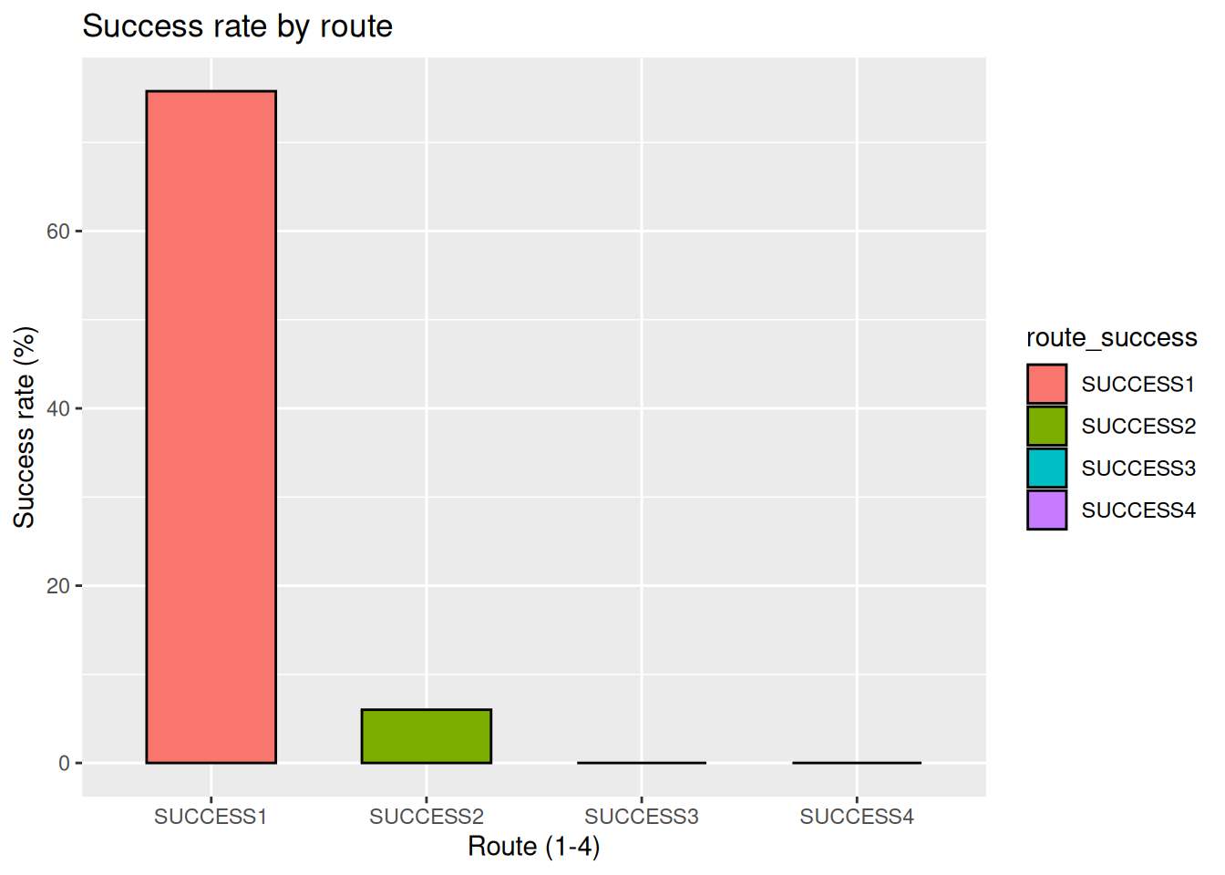
1. What is the most successful route for the expedition for 8000m peaks?

There are 4 different routes enlisted for each peaks, assigned by ROUTE1, ROUTE2, ROUTE3 and ROUTE4. The successful climbing using these routes are stored in corresponding logical vector SUCCESS1, SUCCESS2, SUCCESS3, SUCCESS4. We will use these SUCCESS data along with the exped.8k dataset.

exped.8k |> pivot_longer(cols = c(SUCCESS1, SUCCESS2, SUCCESS3, SUCCESS4),
                           names_to = "route_success",
                           values_to = "success") |>
  group_by(route_success) |>
  summarise(success_rate = (mean(success, na.rm = TRUE))*100) |>
  ggplot(aes(x = route_success, y = success_rate, fill = route_success)) +
  geom_col(width = 0.6, color = "black") +
  labs(
    title = "Success rate by route",
    x = "Route (1-4)",
    y = "Success rate (%)"
  )

2. Which countries has lead the most successful expedition?

Again, we will use the SUCCESS vector; now with the NATION vector; with the exped.data for the details of the all peaks.

exped.data |> filter(SUCCESS1 == TRUE | SUCCESS2 == TRUE | SUCCESS3 == TRUE | SUCCESS4 == TRUE) |>
  count(NATION, sort = TRUE) |>
  ggplot(aes(x = reorder(NATION, n), y = n)) +
  geom_col(fill = "steelblue") +
  geom_text(aes(label = n), hjust = -0.1, size = 3) +
  labs(
    title = "Successful expedition by nation",
    x = "Nation",
    y = "Number of successful expedition"
    ) +
  coord_flip()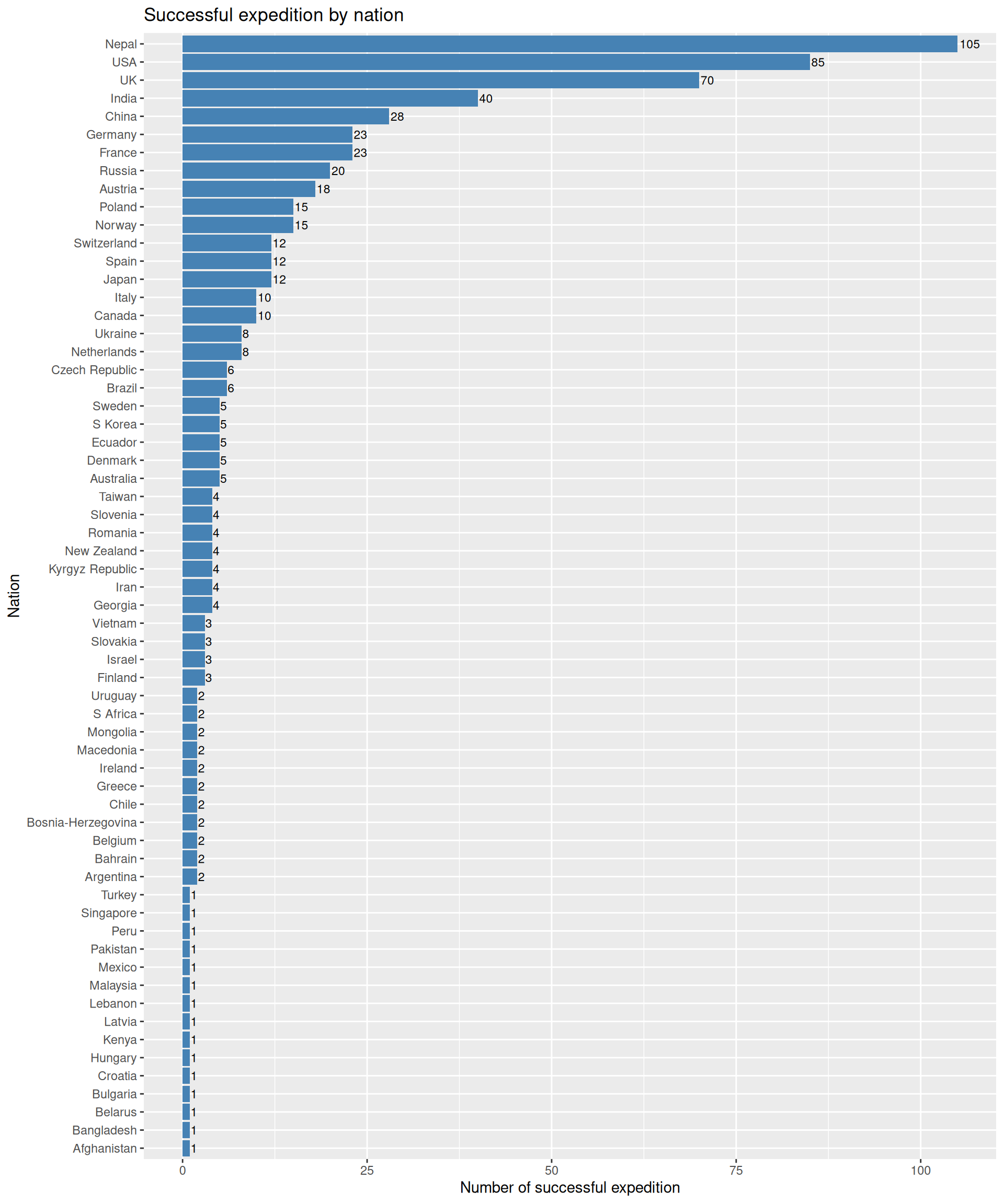

What about the 8000m peaks

We will just use the exped.8k data instead of exped.data from the previous chunk.

exped.8k |> filter(SUCCESS1 == TRUE | SUCCESS2 == TRUE | SUCCESS3 == TRUE | SUCCESS4 == TRUE) |>
  count(NATION, sort = TRUE) |>
  ggplot(aes(x = reorder(NATION, n), y = n)) +
  geom_col(fill = "orangered4") +
  geom_text(aes(label = n), hjust = -0.1, size = 3) +
  labs(
    title = "Successful expedition by nation on 8000m peaks",
    x = "Nation",
    y = "Number of successful expedition"
  ) +
  coord_flip()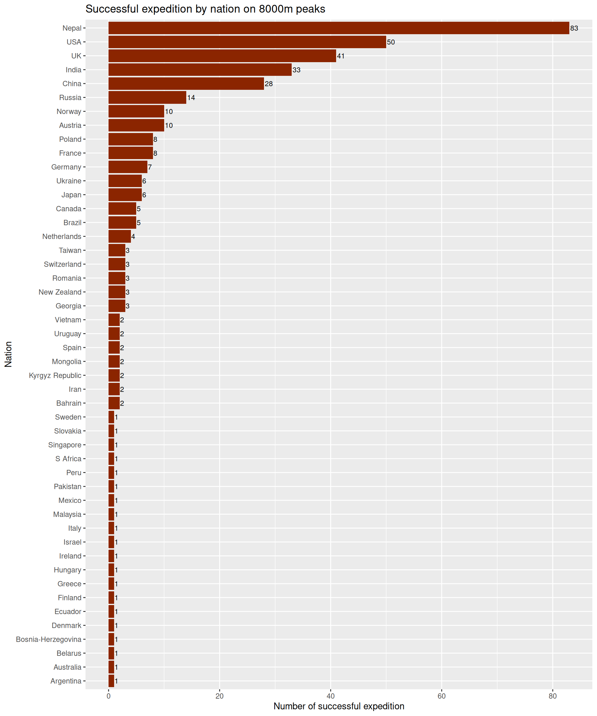

What about the one we actually care about (`Everest`)

exped.8k |> filter(SUCCESS1 == TRUE | SUCCESS2 == TRUE | SUCCESS3 == TRUE | SUCCESS4 == TRUE) |>
  filter(PEAKID == "EVER") |>     #just need to filter the data for Everest
  count(NATION, sort = TRUE) |>
  ggplot(aes(x = reorder(NATION, n), y = n)) +
  geom_col(fill = "lightsalmon3") +
  geom_text(aes(label = n), hjust = -0.1, size = 3) +
  labs(
    title = "Successful expedition by nation on Everest",
    x = "Nation",
    y = "Number of successful expedition"
  ) +
  coord_flip()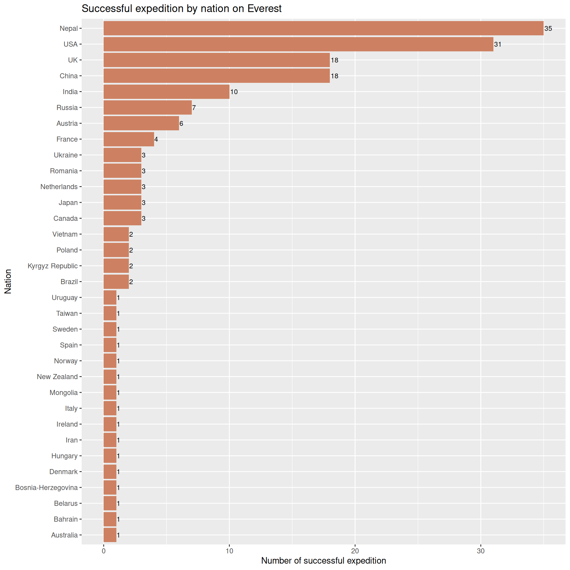

3. How does the travel time vary in different seasons?

exped.data |> filter(!is.na(TOTDAYS), !is.na(SEASON_FACTOR)) |>
  ggplot(aes(x = SEASON_FACTOR, y = TOTDAYS, fill = SEASON_FACTOR)) +
  geom_jitter(aes(colour = SEASON_FACTOR)) +
  scale_color_viridis_d(alpha = 1) +
  labs(
    title = "Expedition duration by season",
    x = "Season",
    y = "Total days of expedition"
  ) +
  theme_minimal() +
  theme(legend.position = "none")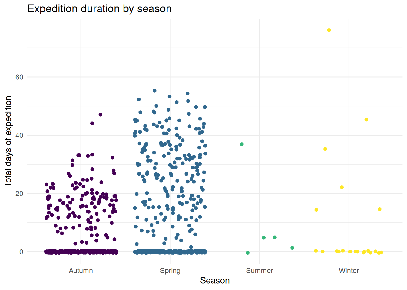

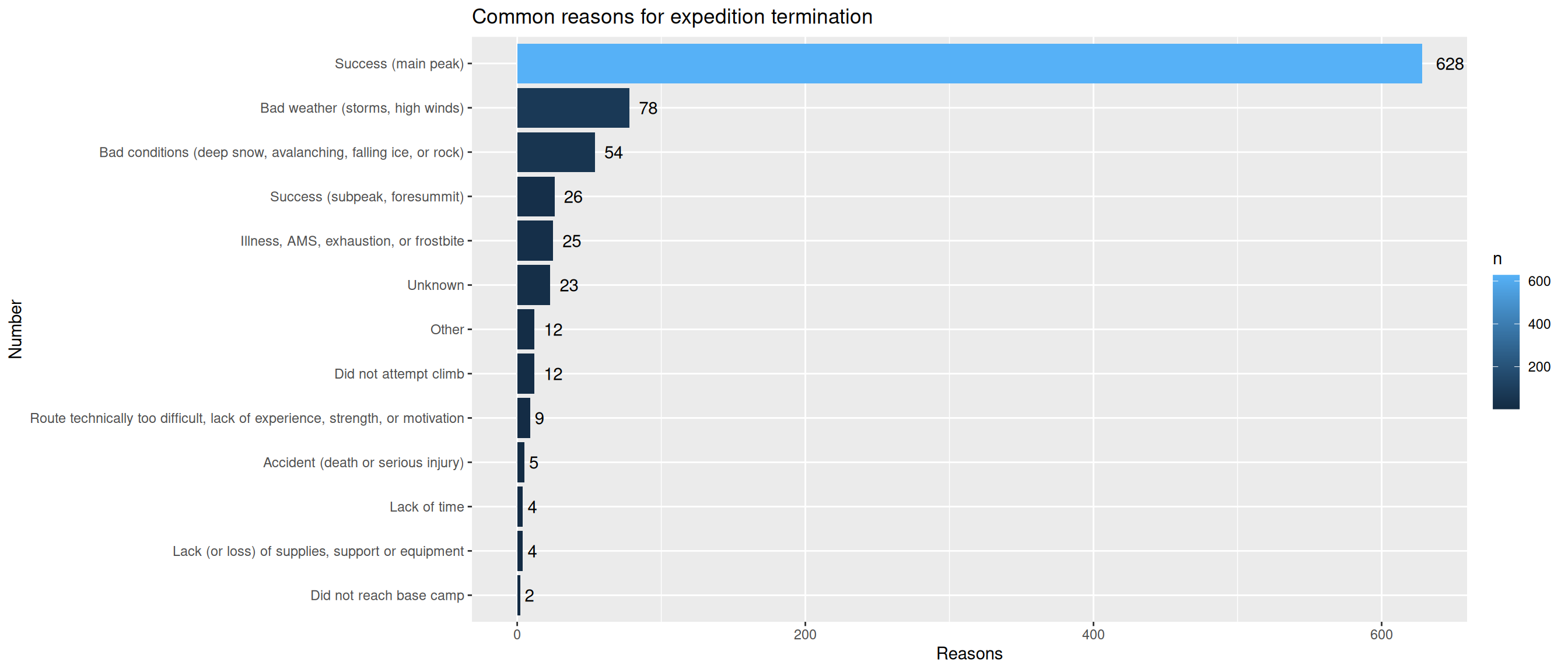
4. Most common reasons for expedition termination

exped.data |> count(TERMREASON_FACTOR, sort=TRUE) |>
  ggplot(aes(x = reorder(TERMREASON_FACTOR,n), y = n, fill = n)) +
  geom_col() + geom_text(aes(label = n, hjust = -0.5)) +
  coord_flip() +
  labs(
    title = "Common reasons for expedition termination",
    x = "Number",
    y = "Reasons"
  )

5. Which peak has the highest fatality rate?

exped.data |> left_join(select(peak.data, PEAKID, PKNAME), by = "PEAKID") |>
  group_by(PKNAME) |>
  summarise(
    expeditions = n(),
    total.deaths = sum(MDEATHS+HDEATHS),
    fatality.rate = total.deaths / expeditions) |>
  arrange(fatality.rate) |>
  slice_max(fatality.rate, n = 10) |>
  ggplot(aes(x = reorder(PKNAME, fatality.rate), y = fatality.rate)) +
  geom_col(fill = "maroon") +
  coord_flip() +
  labs(
    title = "Fatality rate in himalayan peaks",
    x = "Peak name",
    y = "Fatality rate"
  ) +
  theme_minimal()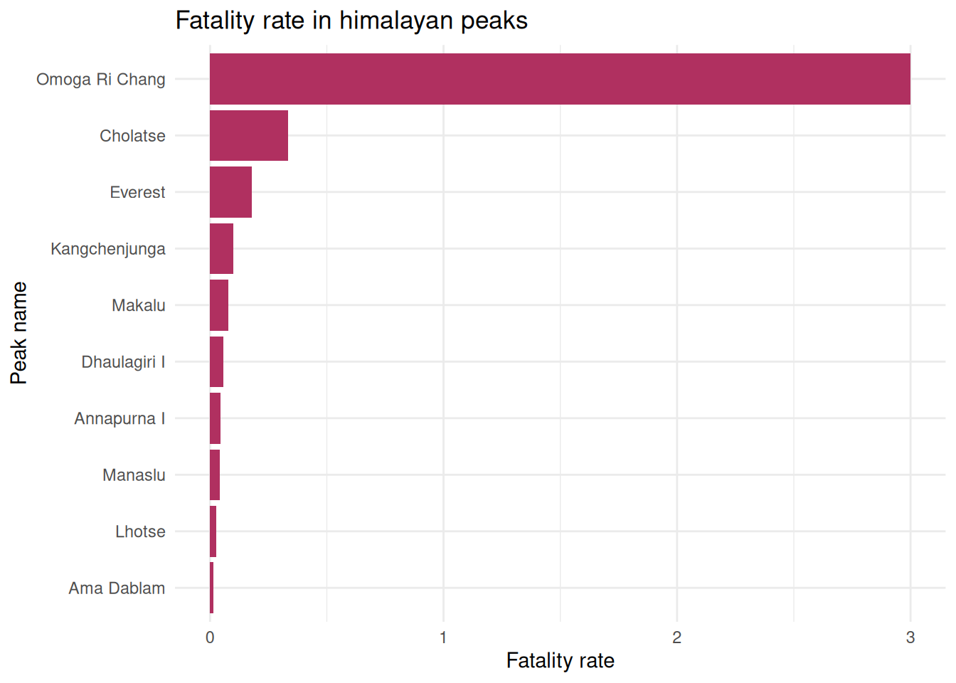

Among the 8000m peaks

exped.8k |> left_join(select(peak.data, PEAKID, PKNAME), by = "PEAKID") |>
  group_by(PKNAME) |>
  summarise(
    expeditions = n(),
    total.deaths = sum(MDEATHS+HDEATHS),
    fatality.rate = total.deaths / expeditions) |>
  arrange(fatality.rate) |>
  #slice_max(fatality.rate, n = 10) |>
  ggplot(aes(x = reorder(PKNAME, fatality.rate), y = fatality.rate)) +
  geom_col(fill = "firebrick3") +
  coord_flip() +
  labs(
    title = "Fatality rate in 8k peaks",
    x = "Peak name",
    y = "Fatality rate"
  ) +
  theme_minimal()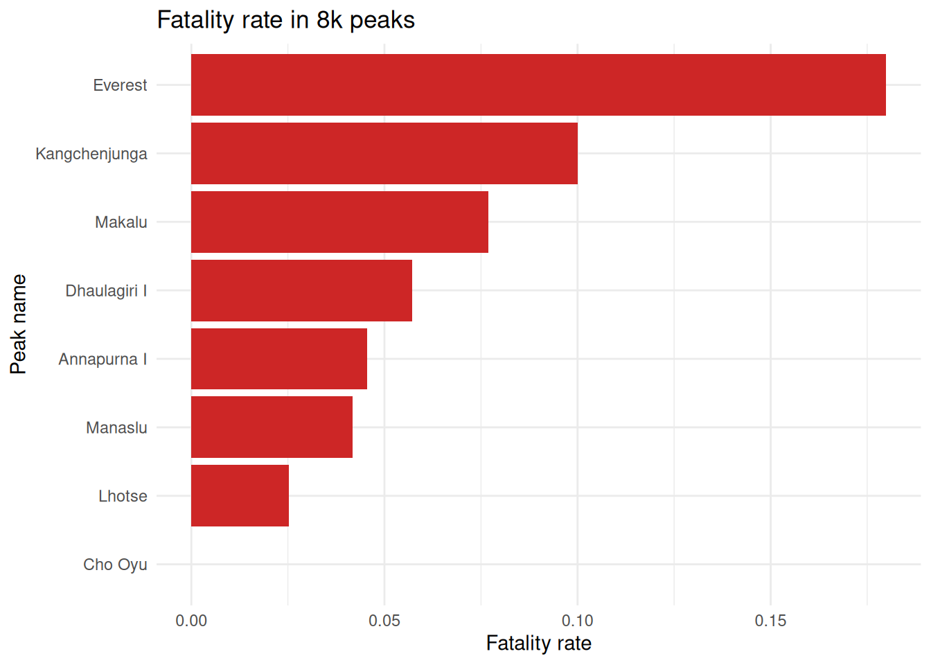

In case of `number of fatalities` on the peaks

exped.data |> left_join(select(peak.data, PEAKID, PKNAME), by = "PEAKID") |>
  group_by(PKNAME) |>
  summarise(total.deaths = sum(MDEATHS+HDEATHS)) |>
  arrange(total.deaths) |>
  slice_max(total.deaths, n = 10) |>
  ggplot(aes(x = reorder(PKNAME, total.deaths), y = total.deaths)) +
  geom_col(fill = "red4") +
  coord_flip() +
  labs(
    title = "Number of deaths in himalayan peaks",
    x = "Peak name",
    y = "No. of death"
  ) +
  geom_text(aes(label = total.deaths), hjust = -.3) +
  theme_minimal()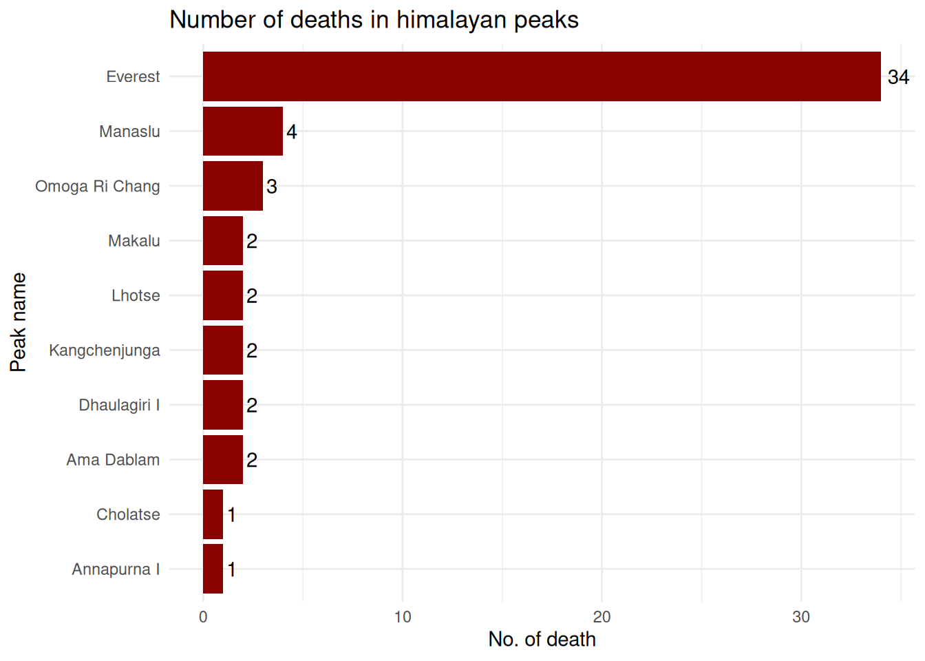

6. Does the use of supplemental oxygen affect the success rate? and death rate?

exped.data |> mutate(success = SUCCESS1 | SUCCESS2 | SUCCESS3 | SUCCESS4,
                     death = MDEATHS + HDEATHS) |>
  group_by(O2USED) |>
  summarise(success.rate = (mean(success, na.rm = TRUE)),
            death.rate = mean(death > 0, na.rm = TRUE)) |>
  pivot_longer(cols = c(success.rate, death.rate), names_to = "names", values_to = "rate") |>
  ggplot(aes(x = O2USED, y = rate, fill = names)) +
  geom_col(position = "dodge") +
  scale_y_continuous(labels = scales::percent) +
  labs(title = "Impact of supplemental Oxygen use on success and deaths",
       x = "Oxygen Used", y = "Rate")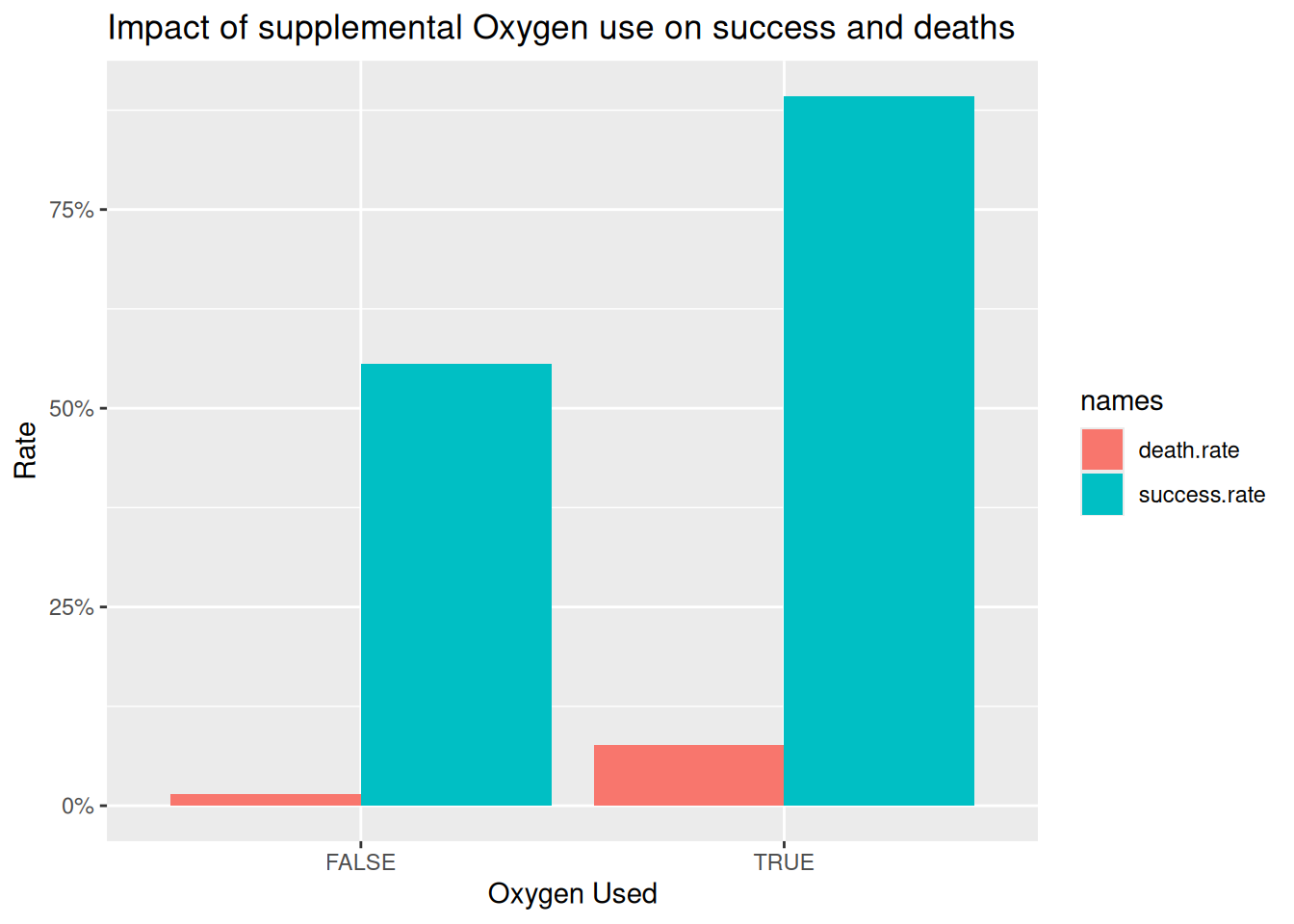

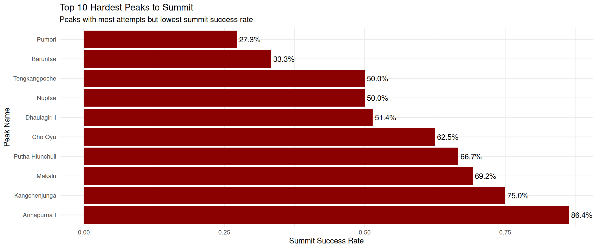
7. Which peaks have the most attempts but lowest summit rate? (Hardest peaks to summit)

exped.data |>
  mutate(success = SUCCESS1 | SUCCESS2 | SUCCESS3 | SUCCESS4) |>
  group_by(PEAKID) |>
  summarise(
    attempts = n(),
    successes = sum(success, na.rm = TRUE),
    summit.rate = successes / attempts) |>
  left_join(select(peak.data, PEAKID, PKNAME), by = "PEAKID") |>
  filter(!is.na(PKNAME), attempts >= 5) |>
  arrange(attempts) |>
  slice_head(n = 10) |>
  arrange(summit.rate) |>
  #slice_head(n = 10) |>
  ggplot(aes(x = reorder(PKNAME, desc(summit.rate)), y = summit.rate)) +
  geom_col(fill = "darkred") +
  geom_text(aes(label = scales::percent(summit.rate, accuracy = 0.1)), hjust = -0.1) +
  coord_flip() +
  labs(
    title = "Top 10 Hardest Peaks to Summit",
    subtitle = "Peaks with most attempts but lowest summit success rate",
    x = "Peak Name",
    y = "Summit Success Rate"
  ) +
  theme_minimal()